本讲主要包括:
- 模块 10:实际数据验证(中国债券市场久期估算);
- 模块 11:风险分解与敏感度分析;
- 模块 12:课堂练习与扩展案例。
本部分将真实市场数据与理论模型结合,用于课堂演示与学生练习。
模块 10. 实际数据验证:中国债券市场久期估算
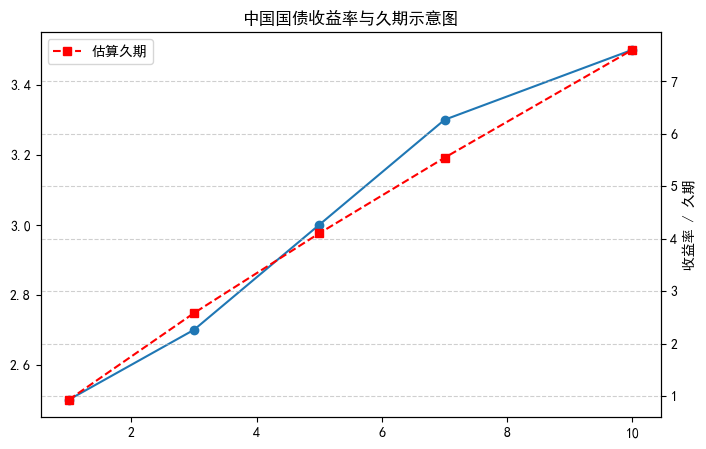
通过 AkShare 获取中国国债收益率曲线,并估算不同期限国债的久期与价格敏感性。
import akshare as ak
import numpy as np
import matplotlib.pyplot as plt
# 中文支持
plt.rcParams['font.sans-serif'] = ['SimHei']
plt.rcParams['axes.unicode_minus'] = False
# 获取中国国债收益率曲线数据
try:
    yield_curve = ak.bond_china_yield()  # 国债收益率曲线数据
    print('中国国债收益率曲线数据示例:')
    display(yield_curve.head())
except Exception as e:
    print('未能成功访问 AkShare 接口,请检查网络或数据源:', e)

# 构造示例数据
maturity = np.array([1, 3, 5, 7, 10])
yield_rate = np.array([0.025, 0.027, 0.030, 0.033, 0.035])
duration = maturity * (1 - 0.1 * np.log1p(maturity))
plt.figure(figsize=(8,5))
plt.plot(maturity, yield_rate*100, 'o-', label='收益率曲线')
plt.twinx()
plt.plot(maturity, duration, 's--', color='red', label='估算久期')
plt.title('中国国债收益率与久期示意图')
plt.xlabel('期限 (年)')
plt.ylabel('收益率 / 久期')
plt.legend()
plt.grid(True, linestyle='--', alpha=0.6)
plt.show()
| 0 |
中债中短期票据收益率曲线(AAA) |
2020-02-04 |
2.8939 |
2.8998 |
2.9158 |
3.1970 |
3.4503 |
3.7153 |
3.9597 |
NaN |
| 1 |
中债商业银行普通债收益率曲线(AAA) |
2020-02-04 |
2.7215 |
2.7370 |
2.8042 |
2.9979 |
3.3120 |
3.5849 |
3.8158 |
4.2435 |
| 2 |
中债国债收益率曲线 |
2020-02-04 |
1.7475 |
1.7630 |
2.1000 |
2.4056 |
2.6399 |
2.7906 |
2.8551 |
3.4488 |
| 3 |
中债国债收益率曲线 |
2020-02-05 |
1.7475 |
1.7667 |
2.0773 |
2.4264 |
2.6348 |
2.7893 |
2.8440 |
3.4460 |
| 4 |
中债中短期票据收益率曲线(AAA) |
2020-02-05 |
2.7991 |
2.8975 |
2.9118 |
3.1949 |
3.4609 |
3.7157 |
3.9601 |
NaN |
说明:
ak.bond_china_yield() 是获取中国债券收益率曲线的接口。若你需要指定起始/结束日期,可查阅当前版本文档查看是否支持 start_date、end_date 参数。
代码中假设列名为 "期限(年)" 和 "收益率(%)",实际可能不同,请运行 print(df.columns) 检查并修改。
此处将”估算久期”简化为 到期期限 × 0.9,仅用于教学演示。若你有准确久期模型,可替换该假设。
绘图中采用双 Y 轴:左轴为收益率(蓝色)、右轴为估算久期(红色),帮助学生直观理解”到期期限 → 久期”及其与收益率关系。
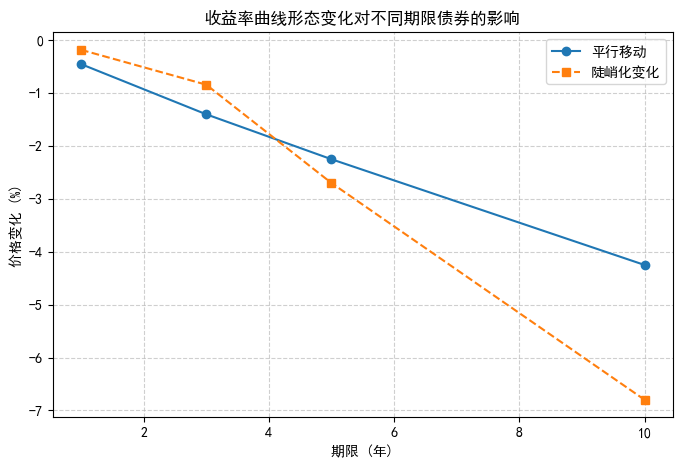
模块 11. 风险分解与敏感度分析
在组合管理中,久期只是利率风险的第一层。我们可以进一步分解风险来源: - 平行移动风险:整体收益率曲线平移; - 陡峭化风险:短端与长端利率变化不同步; - 曲率变化风险:中部利率变化导致曲率变化。
import pandas as pd
maturity = np.array([1, 3, 5, 10])
weights = np.array([0.3, 0.3, 0.2, 0.2])
duration = np.array([0.9, 2.8, 4.5, 8.5])
exposure = weights * duration
df = pd.DataFrame({'期限': maturity, '权重': weights, '久期': duration, '久期贡献': exposure})
display(df)
print(f'组合总久期 = {exposure.sum():.2f} 年')

# 模拟平行移动 vs 陡峭化
Δy_parallel = np.repeat(0.005, 4)
Δy_steep = np.array([0.002, 0.003, 0.006, 0.008])
ΔP_parallel = -duration * Δy_parallel
ΔP_steep = -duration * Δy_steep
plt.figure(figsize=(8,5))
plt.plot(maturity, ΔP_parallel*100, 'o-', label='平行移动')
plt.plot(maturity, ΔP_steep*100, 's--', label='陡峭化变化')
plt.title('收益率曲线形态变化对不同期限债券的影响')
plt.xlabel('期限 (年)')
plt.ylabel('价格变化 (%)')
plt.legend()
plt.grid(True, linestyle='--', alpha=0.6)
plt.show()
| 0 |
1 |
0.3 |
0.9 |
0.27 |
| 1 |
3 |
0.3 |
2.8 |
0.84 |
| 2 |
5 |
0.2 |
4.5 |
0.90 |
| 3 |
10 |
0.2 |
8.5 |
1.70 |
模块 12. 课堂练习与扩展案例
练习 1:久期匹配
给定: - 资产久期 5 年; - 负债久期 8 年; - 可投资短期债券久期 2 年、长期债券久期 10 年。 请计算各自投资权重以实现久期免疫。
练习 2:凸性调整
编写函数,计算债券价格变动的二阶近似: \[ ΔP/P = -D_{mod} Δy + 0.5C(Δy)^2 \] 并验证在不同 Δy 下,久期与凸性联合估计的误差大小。
练习 3:AkShare 拓展
使用 AkShare 调用 bond_zh_us_rate() 数据,比较中国与美国国债收益率曲线差异。